Introduction
Especially in the last decade, we become more familiar with the terms artificial intelligence,
machine learning and data science.
Powerful computers allowed us to perform more
complex statistical operations, from personalizing internet advertisements for each user
to finding out who was the best general in military history (Arsht, 2019). It is important
to clarify these buzzwords before diving into mathematical concepts to inform reader
about this work of field.
Data Types
Plural form of Latin word ”datum”, data, basically means information, information to
observe and make analyzes from. From data science aspect, there are two data types.
- Numerical: Data represented by values. Can either be discrete or continuous.
- Categorical: Data grouped into categories. Can be nominal or ordinal.
With advancement in technology, collecting and processing data become easier. Increments in data
sizes
and ability to use different data sources separated our understanding
of data into two.
Traditional Data
Data that yields a tabular format, therefore each entry is distinct and can be gathered
independently, meaning structured are called traditional data. It is very easy to manipulate
traditional data to with software like Excel or languages like SQL or Python using
pandas library. These manipulations are needed for cleansing.
Big data distinguishes from traditional data along with some of its properties.
Big Data
The name ”big” here leads to a misunderstanding, just being big in volume does not necessarily
mean
that data is a big data, it is about the management as well. Big data has
five characteristic components, also known as 5V’s of big data (vartika02, 2019).
- Volume: This characteristic refers to size of the data. Big data is enormous,
requires
immense storage space.
- Velocity: Big data is gathered continuously. Countless entries take place in the data
sets every fraction of time.
- Variety: Big data can be structured, semi-structured or unstructured.
- Veracity: Working with a pile that huge can lead into confusing situations.
- Value: Data means nothing unless it get modified into something useful.
Big data is separated from traditional data because traditional techniques remains
insufficient, specially designed tools are required. Data sources can be literally anything:
numbers, text, images, videos, audio files etc. Like traditional data, big data also needs to
be cleansed. Table 1 shown below demonstrates some of the differences between traditional
and big data (Rajendran, Asbern, Kumar, Rajesh, & Abhilash, 2016).
| Traditional Data |
Big Data |
| Structured |
Structured, semi-structured or unstructured |
| Small sized |
Needs a lot of storage space |
| Easy to worh with |
Difficult to manipulate |
| Average hardware requirements |
Needs high-end hardware |
| Traditional tools are enough |
Specialized tools are needed |
Table 1: Differences between traditional and big data.
Data Science
Data science is a field of study that analyzes the data collected in various ways and draws
conclusions from them, and makes predictions for the future by examining the patterns.
It is not possible to distinguish the branches of data science completely from each other,
different opinions exists, for example Longbing Cao defines data science as ”data science
= statistics + informatics + computing + communication + sociology + management |
data + environment + thinking” (Cao, 2017).
Business intelligence department uses the data organized by data engineers and analyze
it to gain business insights. Data visualization is a critical skill in this work field,
business
intelligence analysts visualizes the data, measures performance indicators and creates
reports.
To make predictions about future, data scientist use statistical approaches like
- Regression: It is one of the modeling methods used to measure the relationship
between variables. Ranges from simple line fitting to complex structures like forest
models. Used with numerical data.
- Classification: For grouping similar objects into clusters. There are many types
of clustering methods (Xu & Tian, 2015), few of them are centroid-based clustering,
distribution-based clustering, density-based clustering and hierarchical clustering.
Used with categorical data.
- Factor Analysis: Factor analysis is process of explaining observed variables’
variability
with common factors (unobserved variables).
Machine Learning
By being only application of artificial intelligence so far, work principle of algorithms that
enhance themselves by using data and training are called machine learning. Different
machine learning models work better with suited purposes, not every model is capable of
achieving any objective. There are four types of machine learning algorithms: supervised
learning, semi-supervised learning, unsupervised learning and reinforcement learning.
Supervised Learning
Models that work with supervised learning principle learns with features and prediction
data. Initially, data split into two uneven parts: training data and validation data. This
procedure prevents overfitting. Then training data is used for training the model, model
learns relations between features and prediction data. Next, predictions that made by
model using features from validation data are compared to prediction from validation
data to measure errors. Refer Figure 1 for visualization.
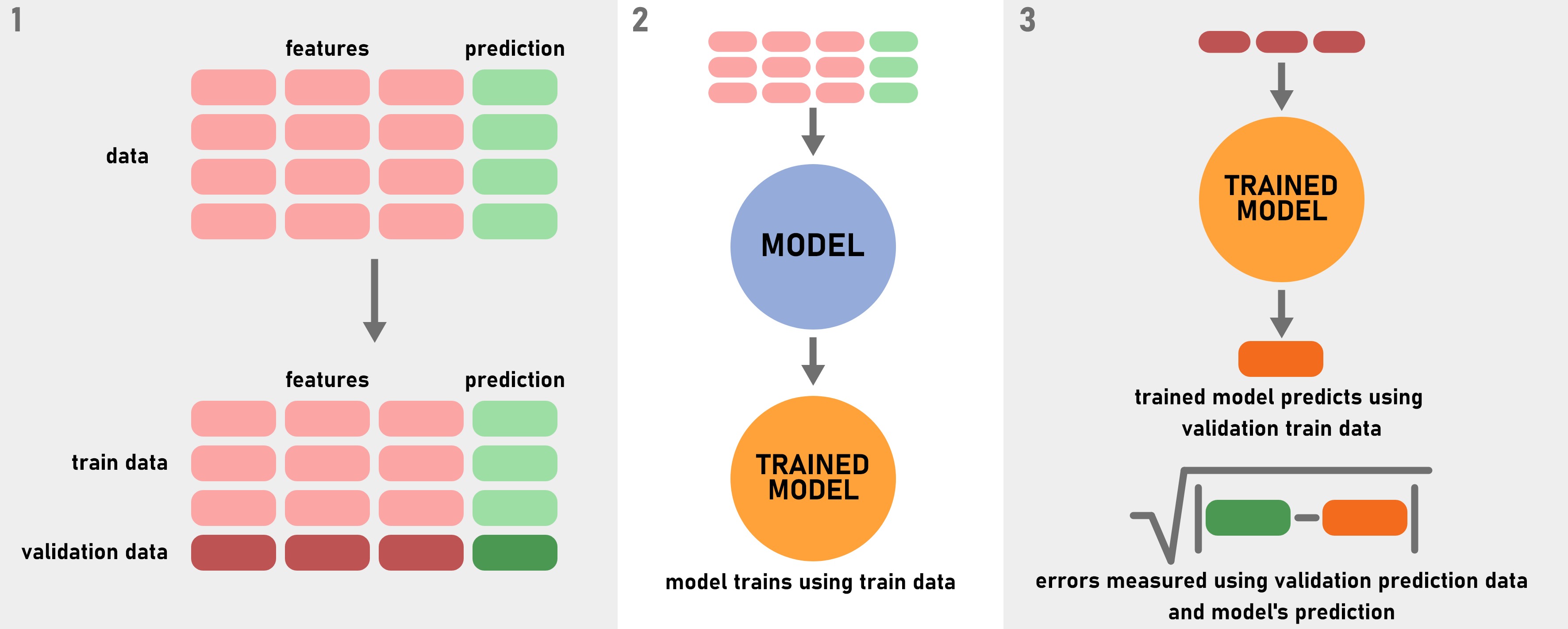
Figure 1: Supervised learning model working principle.
Unsupervised Learning
Unsupervised learning is a learning method used for purposes like grouping or dimensionality
reduction without using initial example. Unlike supervised learning, machine detects
patterns all by itself, using these patterns to group objects into clusters. K-means clustering
is
one the most widely used unsupervised algorithms. It clusters objects around k
centroids by measuring distance between centroid and data, and rearranging the locations
of points, creating Voronoi tessellations. Essentially, k-means learns boundaries between
these tessellations, can be seen in Figure 2.
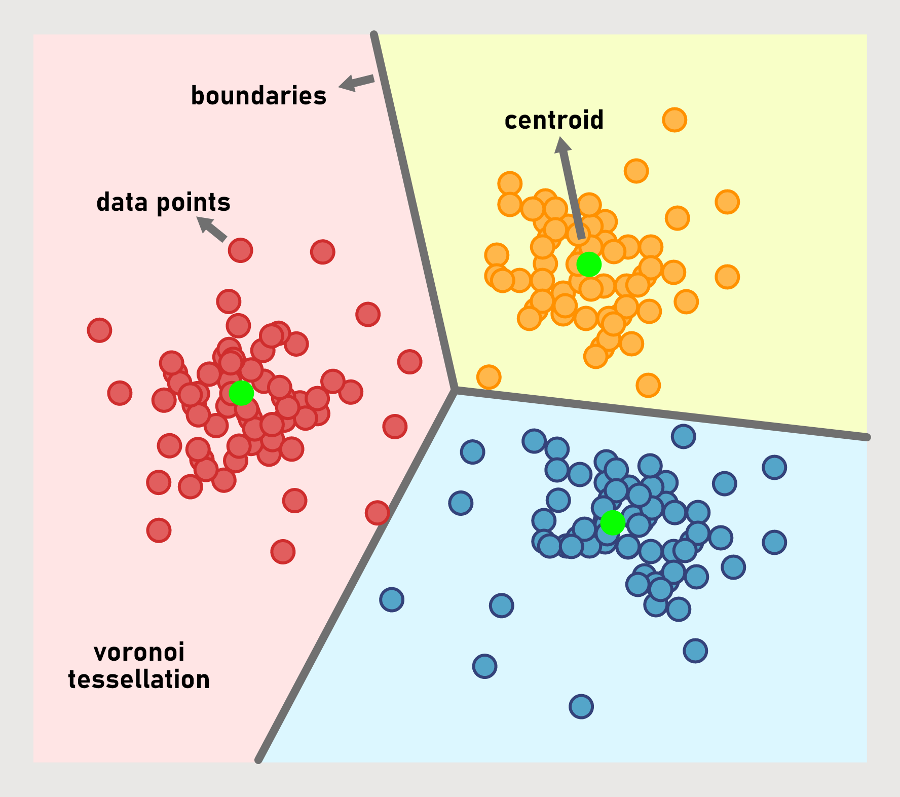
Figure 2: Data clustered with the k-means algorithm, k=3.
Semi-Supervised Learning
Semi-supervised learning models are a blend of supervised and unsupervised learning
models. Used for labelling unlabeled data with the small example of labeled data. Natural
language processing is an example for this learning type.
Reinforcement Learning
Reinforcement learning is a machine learning technique that uses no data, rather rewards
the model to continue on desired path or gives feedback to readjust itself depending on the
outcome. Creating a consistent simulation is a key factor, reinforcement learning works
wonders with simulations with strictly limited rules like chess, go and shogi. Google DeepMind’s
chess bot AlphaZero built on reinforcement learning algorithms, exceeds its
most advanced rival Stockfish within just 4 hours of training (AlphaZero: Shedding new
light on the grand games of chess, shogi and Go, n.d.).
Feature Engineering
Feature engineering is an engineering branch works on acquiring the best outcome from
a machine learning procedure by discovering new features from the raw data.
Along
technical requirements, feature engineers also need common sense to make connection
between features so researching the problem domain could be helpful.
Data visualization is a great tool for future engineering, it can help feature engineers
to detect anomalies, outliers, complicated relations.
Choosing the Right Model
Unlike popular opinion, machine learning models are not magical instruments that capable
of achieving anything, they are tools designed for specialized purposes. Each model has
its advantages and disadvantages, thus selecting the right model is essential.
Creating Features
Features are created by manipulating the raw data. Each model is different, meaning
different kind of approaches are necessary. For example linear models often shows improved
performance with normalized features, normalization especially needed for neural
networks but sometimes tree models can also gain advantage from it. Created features can
be sums, differences, ratios and so on. Even though model can learn it itself, it can still
improve with the particularly implemented feature if it is exclusively important. More
complex the features are, more difficult for model to learn.
Categorical features can either be dropped or encoded.
There are three types of
encoding: ordinal encoding, one-hot encoding or target encoding.
- Ordinal encoding: Assigning values to each categorical data. Used for ordinal
variables.
- One-hot encoding: Creating new columns for each categorical data and filling
these columns with Boolean values, expressing if these variables are a part of the
data or not. Used for nominal variables.
- Target encoding: Replacing categorical value with some numerical value acquired
from the target. Variables low in count may reflect their properties incorrectly, so
acquired numerical property for these variables needs smoothing.
Overfitting and Underfitting
Underfitting is a type of failure when models cannot capture the patterns and put on bad
performance in the training data. This problem generally occurs when the volume of data
remains insufficient, or when the chosen model is not suitable for the data.
Overfitting is type of failure when model performs extremely well in the training
data, but not as well in the validation or test data. This problem occurs when model
capture patterns specific to the given data, too specific that cannot be found in future
predictions. Engineers split data into train data and validation data, train model with
the train data and measure its performance with the validation data to prevent overfitting
from happening. See Figure 1.
Overfitting should be taken into consideration while creating features, joining created feature
to
validation set instead of creating it from validation data as well secures
independence and prevents overfitting.
Cross Validation
While working with considerably small data sets, performance of the model can be boosted
with validating the model by different validation splits. This technique is called
cross-validation.
If the volume of the data is big enough, cross-validation is not necessarily
needed, train data may be able to capture patterns without needing to change it.
Cross-validation
process is visually represented in Figure 3.
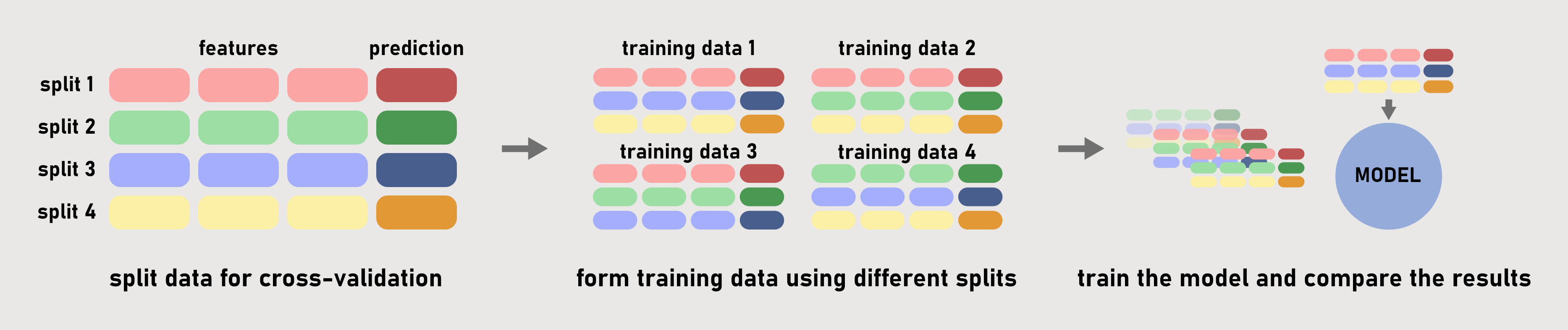
Figure 3: Cross-validation process.
Data Leakage
A data leakage is a kind of failure happens when undesired data is used to train model
along with the training data. Models with data leakage performs extraordinarily well during test
process but fails in real life applications. Data leakage happens in two conditions
Mathematics
When one speaks of artificial intelligence, one first thinks of probability, statistics and
information theory, but that is not all. Behind artificial intelligence lies valuable knowledge
gathered
over millennia. From basic geometry to discrete mathematics, a significant
amount of mathematical knowledge is required to understand how machine learning algorithms work.
Today,
the range of applications for artificial intelligence is immense. It is a
predictive tool in the simplest sense and can be used in any field that requires prediction.
With this mathematical knowledge, machine learning models can be developed into even
more powerful tools, leading to an acceleration of human development. The main
inspiration for this section is the article AI & Mathematics by Shafi (Shafi, 2020).
Basics
Mathematics and programming are like two peas in a pod. Computer algorithms cannot be
constructed without mathematical thinking. Therefore, a significant level of mathematical
maturity is required to understand how machine learning algorithms work. The topics in
this chapter are considered basics because the computations can be performed using basic
mathematical methods.
Geometry
Since data with multiple dimensions can be represented in a Euclidean space, one of the
measurement methods used in machine learning is Euclidean distance. Distances between
data points are used for similarity comparison, clustering, dimensionality reduction, etc.
Euclidean distance formula for n-dimensions is
\begin{align}
d(A,B) = \sqrt{(a_1 - b_1)^2+(a_2 - b_2)^2+ \ldots +(a_n - b_n)^2}
\end{align}
where $A=(a_1, a_2, \ldots , a_n)$ and $B=(b_1, b_2, \ldots , b_n)$.
The center of multiple data points in a space is called the centroid, and the formula for the
centroid of $n$ points is used for clustering, which is
\begin{align}
\left(\frac{x_1+x_2+...+x_n}{n},\frac{y_1+y_2+...+y_n}{n}\right)
\end{align}
Metrics
The performance of a machine learning algorithm is measured by different metrics depending on
the
objective. The metrics used for regression and classification problems differ from each other.
Some
of the regression metrics are explained below.
Mean Squared Error
Mean squared error (MSE) is used to measure the sum of the distances between the data points and
the
regression line. Since the goal of a regression is to fit a line to the data, lower values of
mean
squared error mean that the model is performing better. The formula of the means squared error
is
\begin{align}
\frac{1}{n} \sum_{i=1}^{n}\left(x_{i}-\hat{x}_{i}\right)^{2}
\end{align}
where $n=\text{number of data points}$, $x_{i}=\text{observations}$ and
$\hat{x}_{i}=\text{predictions}$.
Root Mean Squared Error
Mean absolute error (MAE) is a measurement method that works like mean squared error, but
instead of
summing the square root of the differences between predictions and observations, the absolute
values
of the differences are summed. The formula is as follows
\begin{align}
\frac{\sum_{i=1}^{n}\left|x_{i}-\hat{x}_{i}\right|}{n}
\end{align}
R-squared
$R^2$, also called coefficient of determination, is a measurement method for explaining the
variance
between observed and predicted values by the model.
$R^2$ is in the range of $[0,1]$, where $R^2=0$ means that no variability is described by the
regression, and $R^2=1$ means that all variability is described by the regression. The $R^2$ is
usually observed between $(0.2,0.9)$. Note that the value of the $R^2$ varies depending on the
case,
there is no strict interval for a good $R^2$.
To calculate the $R^2$, some terms need to be clarified.
Sum of Squares Total
The sum of squares total (SST or TSS) is the sum of the differences between the observations and
the
mean. It indicates the total variability. The formula is
\begin{align}
\sum_{i=1}^{n} (x_i - \bar{x})^2
\end{align}
Sum of Squares Regression
The sum of squares regression (SSR or ESS) is the sum of the differences between the predictions
and
the mean. It indicates the explained variability. The formula is
\begin{align}
\sum_{i=1}^{n} (\hat{x_i} - \bar{x})^2
\end{align}
Sum of Squares Error
The sum of squares error (SSE or RSS) is the sum of the difference between the observations and
the
predictions. It indicates the unexplained variability. The formula is as follows
\begin{align}
\sum_{i=1}^{n} (\hat{x_i} - {x}_{i})^2
\end{align}
The sum of squares total (SST) is the addition of the sum of squares regression (SSR) and the
sum of
squares error (SSE), which means that the total variability is the sum of explained variability
and
unexplained variability.
\begin{align}
\sum_{i=1}^{n} (x_i - \bar{x})^2 = \sum_{i=1}^{n} (\hat{x_i} - \bar{x})^2 + \sum_{i=1}^{n}
(\hat{x_i} - {x}_{i})^2
\end{align}
And the $R^2$ can be calculated via the following formula
\begin{align}
R^2=\frac{\text{SSR}}{\text{SST}}
\end{align}
Adjusted R-squared
Adjusted R-squared, abbreviated as $\bar{R}^2$, is a measurement method derived from $R^2$. It
incorporates the sample size and the number of independent variables in addition to $R^2$ and is
calculated using the following formula.
\begin{align}
\bar{R}^2 = 1-(1-R^2)\frac{n-1}{n-p-1}
\end{align}
Where $n$ is the sample size, which can also be viewed as the number of rows, and $p$ is the
number
of independent variables, which indicates the number of features. Since the $\bar{R}^2$
penalizes
the excessive use of variables, it is always smaller than the $R^2$.
\begin{align}
\bar{R}^2 < R^2 \end{align} And some of the classification metrics are explained below.
Accuracy, Precision and Recall
Accuracy, precision, and recall are the
classification metrics calculated using the confusion matrix. The confusion matrix is a
graph that shows the correct and incorrect predictions of the model. The rows show the
predictions, while the columns show the observations. See Table 2 for clarification.
|
Positive observations |
Negative observations |
| Positive predictions |
True positives (TP) |
False positives (FP) |
| Negative predictions |
False negatives (FN) |
True negatives (TN) |
Table 2: The confusion matrix.
Accuracy is the ratio of total correct predictions to all predictions.
\begin{align}
\text{Accuracy}=\frac{TP+TN}{TP+TN+FP+FN}=\frac{\text{correct predictions}}{\text{all
predictions}}
\end{align}
The problem with accuracy is with unevenly distributed data sets. The measurement of
accuracy is
inadequate when the negative or positive observations make up the bulk of the data. For
example,
consider an observation set consisting of the following elements.
observations = [A, A, A, A, A, A, A, A, B]
If a model makes a prediction consisting entirely of A's,
predictions = [A, A, A, A, A, A, A, A, A]
the accuracy would be $90\%$. The model completely ignores one of the observations and still
achieves very high accuracy.
The formula of the precision is
\begin{align}
\text{Precision}=\frac{TP}{TP+FP}=\frac{\text{true positives}}{\text{all positive
predictions}}
\end{align}
If the positive predictions are more important for the goal, it is better to use precision
as a
measure.
And the formula of the recall is
\begin{align}
\text{Recall}=\frac{TP}{TP+FN}=\frac{\text{true positives}}{\text{all positive
observations}}
\end{align}
If the negative predictions are more important for the objective, recall is a better
measurement
method. To avoid the misconceptions caused by the unbalanced data sets, F1-score is used.
F1-score
The F1-score is a classification metric calculated based on precision and recall. In real-world
machine learning applications, the data sets encountered are often unbalanced. The F1-score is
used
to remove the misunderstandings caused by the imbalanced data by averaging the precision and
recall.
The F1-score is calculated as follows.
\begin{align}
F_{1}=\frac{2\cdot\text{precision}\cdot\text{recall}}{\text{precision}+\text{recall}}
\end{align}
Calculus
Infinitesimal calculus, which has its roots in the researches of Newton and Leibniz (Rosenthal,
1951), has not lost its importance since the day of its discovery. Machine learning algorithms
aim
to optimise their objective functions as the parameters change, and the role
of the calculus is to represent the performance of the algorithm (Brownlee, Cristina, &
Saeed, 2022). In addition to the optimization methods and the objective functions, another
application of this topic is to ensure the nonlinear behaviour in regression problems
using the activation functions. Also, this section explores how Fourier series are used in
time series analysis
Objective Functions
The goal of machine learning algorithms is to optimize their objective functions. Depending on
the
model, it may be beneficial to increase or decrease the value of the objective
functions. Supervised learning models aim to minimize the loss function, while the goal
of reinforced learning models is to maximize the reward function.
L2-norm Loss
The L2 norm loss or squared loss is a widely used loss function in regression problems. It can
be
calculated like the mean squared error.
\begin{align}
\sum_{i}{}(y_i - t\hat{y}_i)^2
\end{align}
It is basically the Euclidean distance between the observations and the predictions, hence the
name
norm.
Cross-entropy
Cross entropy is a loss function used in classification problems. The classification metrics
mentioned in the previous section are discrete, since these metrics are nothing more than a
ratio of
counts. Cross-entropy, on the other hand, is continuous, and this continuity is required for
gradient descent algorithms.
The formula of the cross-entropy is
\begin{align}
L(\hat{y}_{i},y_{i})=-\sum_{i}{} y_{i} ln\hat{y}_{i}
\end{align}
where $y_{i}=\text{target value}$ and $\hat{y}_{i}=\text{predicted value}$. The value of
cross-entropy decreases with better prediction. For example, consider a visual data set
consisting
of dog, cat and bird images, where the target vectors are defined as follows.
dog = [1, 0, 0]
cat = [0, 1, 0]
bird = [0, 0, 1]
If the model makes a prediction based on a picture of a cat and calculates that the animal in the
picture is 20% dog, 40% cat, and 40% bird
prediction = [0.2, 0.4, 0.4]
the cross-entropy would be
\begin{align}
L(\hat{y}_{i},y_{i})=-0\cdot ln0.2-1\cdot ln0.4-0\cdot ln0.4=0.91
\end{align}
Loss functions are used to reduce variance by training the model with the training data. Metrics, on
the other hand, are used to reduce bias calculated using the test data.
Activation Functions
As the relationships between variables become more complex, linear approximations are
no longer sufficient. In neural networks, activation functions are used to convert linear
combinations into nonlinear ones. This process is necessary to stack the layers, because a
network consisting only of linear combinations is nothing more than a linear regression.
For a better explanation, see Figure 4.
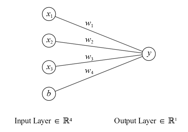
Figure 4: A rather small neural network with inputs and weights.
In this model, $y$ is
\begin{align}
y=x_1 w_1 + x_2 w_2 + x_3 w_2 + b w_4
\end{align}
It can be stated that neural networks consisting only of input and output layers are linear
regression. For further reading, below are some of the most commonly used activation functions.
Sigmoid
The sigmoid function, also known as the logistic function, is an activation function used in
neural
networks. Since the sigmoid function ranges between $(0,1)$, it is generally used when the
desired
prediction is to be a probability. Its formula is as follows.
\begin{align}
\sigma(a)=\frac{1}{1+e^{-a}}
\end{align}
Derivatives of the activation functions are used in backpropagation. The derivative of the
sigmoid
function is
\begin{align}
\frac{\partial \sigma(a)}{\partial a}=\sigma(a)(1-\sigma(a))
\end{align}
Python code that plots the sigmoid function is given below. See Figure 5.
a = np.arange(-5, 5, 0.01)  # defining a range to plot the function on
sigmoid = 1 / (1 + np.exp(-a))  # the sigmoid function
plt.axvline(x=0, color="red")
plt.axhline(y=0, color="red")  # x and y axis
plt.plot(a, sigmoid, lw=3) # plotting the sigmoid function
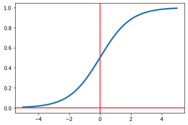
Figure 5: The sigmoid function.
tanh
The hyperbolic tangent function is another activation function used in neural networks. The
output
of the $tanh$ function is between $(-1,1)$. Its formula is
\begin{align}
tanh(a)=\frac{e^a - e^{-a}}{e^a + e^{-a}}
\end{align}
And the derivative of the $tanh$ function is
\begin{align}
\frac{\partial tanh(a)}{\partial a}=\frac{4}{(e^a + e^{-a})^2}
\end{align}
See Figure 6 for this function's graph.
a = np.arange(-5, 5, 0.01)  # defining a range to plot the function on
tanh = (np.exp(a) - np.exp(-a)) / (np.exp(a) + np.exp(-a))  # the tanh function
plt.axvline(x=0, color="red")
plt.axhline(y=0, color="red")  # x and y axis
plt.plot(a, tanh, lw=3)  # plotting the tanh function
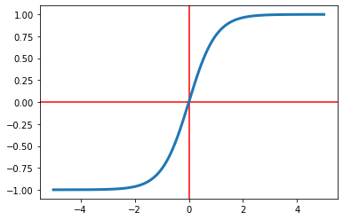
Figure 6: The tanh function.
ReLU
The rectified linear unit function, \textit{ReLU} for short, is an activation function used when
all
values below $0$ are considered unimportant. It ranges between $(0,\infty)$ and sets all values
below
$0$ to $0$. The formula of the ReLU function is
\begin{align}
relu(a)=max(0,a)
\end{align}
And its derivative is
\begin{align}
\frac{\partial \operatorname{relu}(a)}{\partial a}=\left\{\begin{array}{l}
0, \text { if } a \leq 0 \\
1, \text { if } a>0
\end{array}\right.
\end{align}
Python code given below plots the ReLU function and its graph can be seen in Figure 7.
a = np.arange(-5, 5, 0.01)  # defining a range to plot the function on
relu = np.maximum(0, a)  # the relu function
plt.axvline(x=0, color="red")
plt.axhline(y=0, color="red")  # x and y axis
plt.plot(a, relu, lw=3)  # plotting the relu function
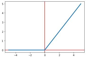
Figure 7: The ReLU function.
softmax
The softmax activation function is used to transform imported values into an accurate
probability
distribution. Thus, the sum of the outputs of the softmax activation function is equal to $1$.
The
formula is
\begin{align}
\sigma_{\mathrm{i}}(a)=\frac{e^{a_{i}}}{\sum_{j} e^{a_{j}}}
\end{align}
And the derivative of the softmax function is
\begin{align}
\frac{\partial \sigma_{i}(a)}{\partial a_{j}}=\sigma_{i}(a)\left(\delta_{i
j}-\sigma_{j}(a)\right)
\end{align}
where $\delta_{i j}$ is the Kronecker delta, i.e., $i=j$, $\delta_{i j}=1$ and if $i\neq j$,
$\delta_{i j}=0$.
The following Python code defines the softmax function and converts the input values into
probabilities.
softmax = lambda x: np.exp(x) / np.exp(x).sum()  # defining the softmax function
inputValues = [12, 3, 29, 14, 8] # random values
outputValues = softmax(inputValues)
The output values are
[4.13993628e-08, 5.10908725e-12, 9.99999652e-01, 3.05902214e-07, 7.58255779e-10].
And the sum of the probabilities can be calculated as follows.
sum(outputValues)
The output is
1.
Fourier Series
Fourier series are used as features in time series analysis. The goal is to let the model
learn from these Fourier features by breaking down the series into sine and cosine waves.
All types of time series analysis performed using sinusoids are called Fourier analysis
(Bloomfield, 2004)
The Figure 8 below nicely illustrates how the summation of Fourier features estimates
seasonality (Holbrook, 2021).
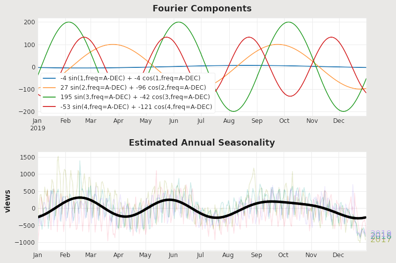
Figure 8: Sine and cosine waves can be used to determine seasonality.
Fourier features can be implemented via statsmodels library. This library includes the
CalenderFourier method. The code block below generates 4 sine and cosine pairs for monthly
seasonality.
from statsmodels.tsa.deterministic import CalendarFourier

fourier = CalendarFourier(freq="M", order=4)
Optimization
Machine learning is all about optimization. The main goal of machine learning algorithms
is to change the values of the weights to achieve the best result of the loss function and
metrics. This goal is achieved with the gradient descent algorithm, which has been further
developed over the years.
Gradient Descent
Gradient descent is an iterative process used to find minima or maxima of a function. In machine
learning, gradient descent is used as an optimization algorithm. The updated value of $x$ is
calculated with
\begin{align}
x_{i+1}=x_i - \eta f'(x_i)
\end{align}
where $\eta$ is the learning rate. The gradient descent algorithm can also be applied to higher
dimensions. Consider a linear regression model $x_i w + b = \hat{y}_i \rightarrow y_i$ with the
loss
function $L$. The updated values for the weight and the bias are calculated using the following
formulas.
\begin{align}
w_{i+1}&=w_i - \eta \nabla_w L(\hat{y},y) \\
b_{i+1}&=b_i - \eta \nabla_b L(\hat{y},y)
\end{align}
The gradient descent algorithm is demonstrated in Figure 9.

Figure 9: The gradient descent algorithm.
Stochastic Gradient Descent
One method for speeding up the process of updating
weights is batching. Instead of updating the weights after each epoch, the data set is split
into batches to update the weights multiple times in a single epoch. With this approach,
computers are able to train different batches using CPU cores. This algorithm is called
stochastic gradient descent. The term ”stochastic” refers to the randomness of the batches
selected.
Momentum
The gradient descent algorithm alone sometimes fails to find a global minimum, but only the
local
minima (see Figure 10). Stopping the optimization at an extrema point can be prevented by adding
momentum to the gradient descent. Recall the formula for gradient descent at moment $t$.
\begin{align} \label{gd}
w(t+1) = w(t)- \eta\frac{\partial L}{\partial w}(t)
\end{align}
Putting the descent at time $(t-1)$ into the formula for the gradient descent and multiplying it
by
the constant $\gamma$, the following formula is acquired.
\begin{align}
w(t+1) = w(t) - \eta\frac{\partial L}{\partial w}(t) - \gamma\eta\frac{\partial L}{\partial
w}(t-1)
\end{align}
where $0\leq \gamma \leq 1$. Multiplying the previous descent by a number between 0 and 1
reduces
the effectiveness of the previous steps with each iteration.
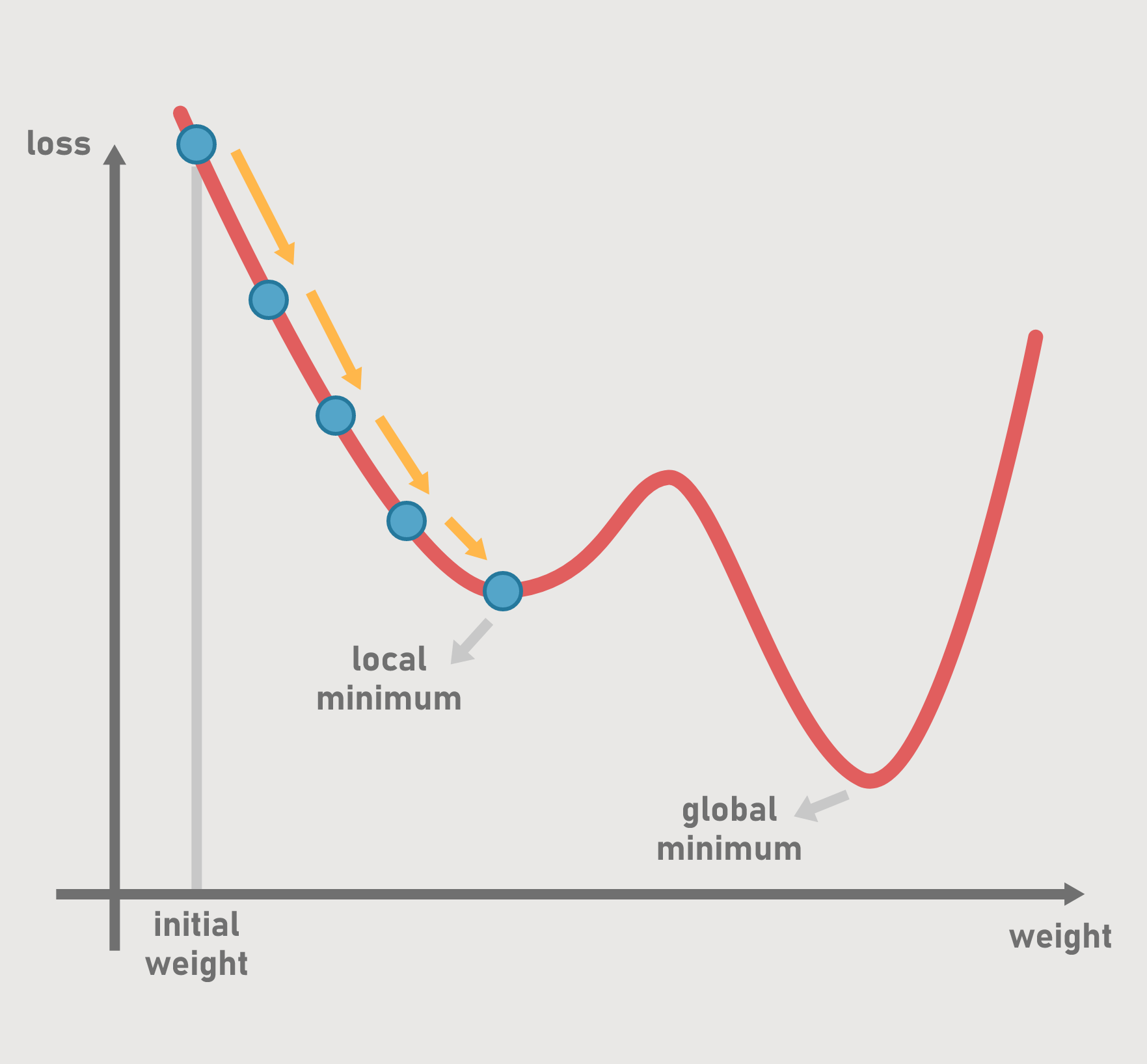
Figure 10: The gradient descent might remain insufficient.
Learning Rate
The learning rate is a parameter that determines the speed of convergence of the algorithm to
the
extrema point. It is important to choose an appropriate learning rate that is not too high and
not
too low, since a very high learning rate will cause oscillation and a very low learning rate
will
cause the algorithm to iterate continuously. The learning rate is denoted by $\eta$.
Updating the learning rate across epochs improves algorithm performance. Small learning rates
may
not be necessary at the beginning, but to prevent the gradient descent algorithm from
oscillating,
the learning rate must eventually be lowered. This process is called a learning rate schedule.
Piecewise Learning Rate
The piecewise learning rate updates the learning rate for a fixed number of epochs. For example,
starting from a learning rate $\eta=0.1$ yields the following piecewise learning rate schedule.
- $\eta=0.1$ for the first 10 epochs
- $\eta=0.05$ for the following 10 epochs
- $\eta=0.025$ for the following 10 epochs
- $\eta=0.001$ until the last epoch
Exponential Learning Rate
The exponential learning rate updates the learning rate according to the following formula.
\begin{align}
\eta=\eta_0 e^{n/c}
\end{align}
where $n=\text{number of epochs}$ and $c=\text{a constant}$. $c$ is a hyperparameter
proportional to
the number of epochs.
Adaptive Learning Rate Schedules
The learning rate can also be dynamically updated for individual weights. This method helps to
reduce the training time of
the model (Okewu, Misra, & Lius, 2020). Some of the adaptive learning rate schedules
are listed below.
Adaptive Gradient Algorithm
Adaptive gradient algorithm, or AdaGrad, is an
adaptive learning rate schedule that dynamically varies the learning rate as a function of
feature frequency (Lydia & Francis, 2019). The formula of the adaptive gradient algorithm
can be obtained by manipulating the momentum formula.
\begin{align}
w(t+1)-w(t)&=-\eta\frac{\partial L}{\partial w}(t) \\
\Delta w &= -\eta\frac{\partial L}{\partial w}(t)
\end{align}
Replacing $w$ by the weight index $w_i$ and dividing the learning rate $\eta$ by $\sqrt{G_i (t)
+
\epsilon}$, the formula of the adaptive gradient algorithm is obtained.
\begin{align} \label{adagrad}
\Delta w_i (t)=-\frac{\eta}{\sqrt{G_i (t)}+\epsilon}\frac{\partial L}{\partial w_i}(t)
\end{align}
where
\begin{align}
G_i (t) = G_i (t-1) + \left(\frac{\partial L}{\partial w_i}(t)\right)^2
\end{align}
The reason for the absence of $\epsilon$ in the denominator is to avoid division by zero, since
$G_i
(0)=0$.
Root Mean Square Propagation
Root mean square propagation, or RMSprop in short, is an adaptive learning rate schedule similar
to
AdaGrad with a different $G_i (t)$ function. The formula is the same as the formula of AdaGrad,
where
$G_i (t)$ is
\begin{align}
G_i (t) =\gamma G_i (t-1) + (1-\gamma)\left(\frac{\partial L}{\partial w_i}(t)\right)^2
\end{align}
Where $\gamma$ is a hyperparameter. Note that $G_i (t)$ in RMSprop is not monotonically
decreasing
like the AdaGrad algorithm.
Adaptive Moment Estimation
Adaptive moment estimation (ADAM) combines momentum with adaptive learning rate schedules. The
goal
of adaptive moment estimation is to gain control over step sizes to solve problems caused by the
gradient descent algorithm alone. The formula for adaptive moment estimation is
\begin{align}
\Delta w_i (t)=-\frac{\eta}{\sqrt{G_i (t)}+\epsilon}M_i (t)
\end{align}
where
\begin{align}
M_i (t)=\gamma M_i (t-1)+(1-\gamma)\frac{\partial L}{\partial w_i}(t)
\end{align}
Initialization
Randomly selecting initial values for the weights from the standard normal distribution or the
uniform distribution causes models with nonlinear activation
functions to perform poorly, especially models
with activation functions such as sigmoid and tanh, because the input values around the
mean exhibit linear behaviour (Glorot & Bengio, 2010). Xavier initialization or Glorot
initialization, named after Xavier Glorot, helps improve the performance of machine learning
models
by using the number of input and output values to determine the distribution
parameters.
Uniform Xavier Initialization
The selection of the weights from a uniform distribution in the range of $[-x,x]$, where $x$
stands
for
\begin{align}
x=\sqrt{\frac{6}{\text{number of inputs}+\text{number of outputs}}}
\end{align}
Normal Xavier Initialization
The selection of the weights from a normal distribution where $\mu=0$ and
\begin{align}
\sigma=\sqrt{\frac{6}{\text{number of inputs}+\text{number of outputs}}}
\end{align}
Algebra
Counting things has been a part of our lives since the beginning of the human era (Garding
& Tambour, 2012). Therefore, it is not surprising that algebra is a part of computer
programming, that is, machine learning.
Vectors, matrices, and tensors are used for
computations, and these structures are often called arrays in programming.
Kernels
Algebra is one of the fundamental mathematical topics of image processing. Actually, images in
digital media are multidimensional arrays. In order for image processing algorithms to learn,
different types of features must be obtained from the images. Matrices that extract features
from an
image by computing weighted sums are called kernels. An example of a kernel used for edge
detection
is given below.
\begin{align} \label{kernel}
A=\left[\begin{array}{rrr}
-1 & -1 & -1 \\
-1 & 8 & -1 \\
-1 & -1 & -1
\end{array}\right]
\end{align}
Consider an image given as
\begin{align} \ label{imagematrix}
B=\left[\begin{array}{rrr}
2 & 6 & 3 \\
2 & 2 & 4 \\
7 & 1 & 1
\end{array}\right]
\end{align}
The formula for the weighted sum is
\begin{align} \label{weightedsum}
\sum_{i}{} \sum_{j}{} a_{ij} b_{ij}
\end{align}
And the weighted sum obtained from the image is
\begin{align}
&=((-1)\cdot 2 + (-1) \cdot 6 + (-1) \cdot 3) \\
&+((-1) \cdot 2 + 8 \cdot 2 + (-1) \cdot 4) \\
&+((-1) \cdot 7 + (-1) \cdot 1 + (-1) \cdot 1) \\
&=-10
\end{align}
Tensors
Tensor is a general mathematical term for arrays. In fact, vectors and matrices are tensors
with one and two dimensions (Kan, 2021). However, not every matrix is considered a tensor
because
tensors are considered dynamic objects (Steinke, 2017)
Discrete Mathematics
The computers we use in our daily lives are digital, and digital computers are known to
perform calculations on discrete systems (The Editors of Encyclopaedia Britannica, 2020),
so it is no wonder that discrete mathematics is a part of computer programming, hence
machine learning.
Graph Theory
One way to visualize the relationships between entities is to use graphs. Graph theory is
often used to represent neural networks (Figure 11) and decision trees (Figure 12).
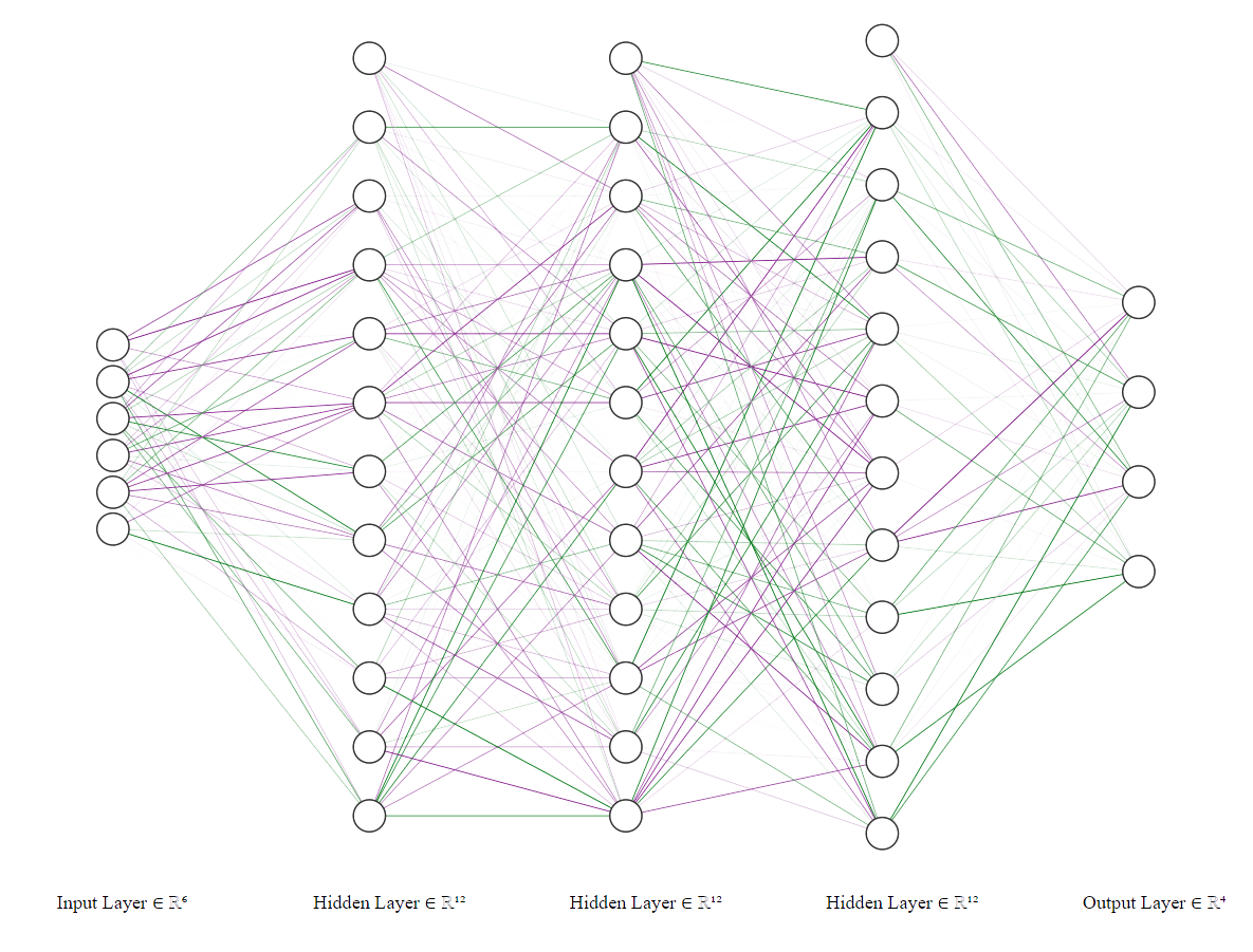
Figure 11: An artificial neural network.
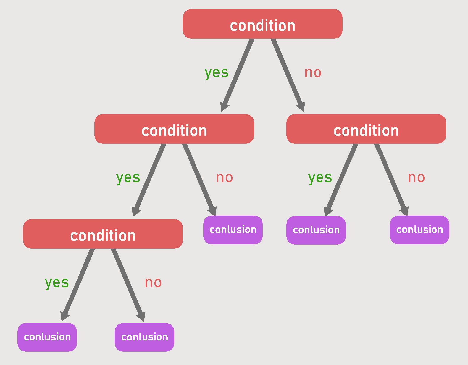
Figure 12: A decision tree.
Time Complexity
In computer science, one way to measure the efficiency of an algorithm is to calculate its
time complexity. The running speed of algorithms strongly affects the training time, since
machine learning is an iterative process.
Using the numbers n for the training examples, d for the dimensions, and k for the
neighbours, the training time complexities of some machine learning algorithms are given
as (Kumar, 2021).
- K nearest neighbors: $O(knd)$
- Logistic regression: $O(nd)$
- Decision tree: $O(nlog(n)d)$
- Random forest: $O(nlog(n)dk)$
Probability Theory
By observing nature, patterns can be identified, and probability methods can be used to
make predictions about the future based on these patterns. Because machine learning algorithms
are
trained with observations to compute probabilities, this area of mathematics
takes a critical role in artificial intelligence applications. The correctness of predictions
made by machines is measured with confidence intervals to see how certain they are
(DasGupta, 2011). However, this section consists of
Bayes’ theorem, expected value and variance, distributions, and the expected value and
variance of these distributions, which form a basis for statistics.
Bayes’ Theorem
Bayes’ theorem is a mathematical equation used to calculate conditional probability. In
1763, Thomas Bayes discovered that the theorem expresses the likelihood of an event that
is affected by another event (Bayes’ theorem, 2022). If $A$ and $B$ are the events and, $P(A)$
and
$P(B)$ are the probabilities of these events, Bayes' theorem is as follows.
\begin{align}
P(A \mid B)=\frac{P(B \mid A) \cdot P(A)}{P(B)}
\end{align}
Where, $P(A \mid B)$ is the probability of $A$ being true when $B$ is true, and $P(B \mid A)$ is
the
probability of $B$ being true when $A$ is true.
Expected Value and Variance
There are two types of variables: Discrete and continuous. Discrete variables can be counted,
that
is, they are finite. Continuous variables, on the other hand, cannot be counted, so it is only
possible to measure them in an interval.
The expected value is the weighted average of the possible values a variable can take. Since $X$
is
a random variable, the expected value of $X$ is denoted by $E[X]$. The probability function of
$X$
is $p(x)$ and the probability density function of $X$ is $f(x)$. The formulas for the expected
value
are given below.
\begin{align}
E[X]&=\sum xp(x)\:\:\: \text{for discrete variables} \\
E[X]&=\int _{-\infty }^{\infty }xf(x)dx\:\:\:\text{for continuous variables}
\end{align}
Some properties of the expected value are:
- $E[X]=\mu, \quad (\mu \: \text{is the mean of} \: X)$
- $E[aX+b]=aE[X]+b$
- $E[X + Y] = E[X] + E[Y]$
- $E[XY] = E[X]E[Y], \quad \text{(X and Y are independent variables)}$
Another fundamental element of probability is the variance, which is calculated using the expected
value.
The variance is a measure of variability, it indicates how wide a distribution is. Since $X$ is a
random variable, the variance of $X$ is given as $Var(X)$. The formulas are
\begin{align}
Var(X)&=\sum (x-\mu)^2p(x) \quad \text{for discrete variables} \\
Var(X)&=\int _{-\infty}^{\infty}(x-\mu)^2f(x)dx \quad \text{for continuous variables}
\end{align}
Some properties of the variance are
- $Var(X)=\sigma^2, \quad (\sigma^2 \: \text{is the variance of} \: X)$
- $Var(aX+b)=a^2Var(X)$
The variance can also be expressed as $E[X^2]-E^2[X]$. Can be proved using the properties of the
expected value.
\begin{align}
Var(X)&=E[(X-E[X])^2] \\
&=E[X^2-2XE[X]+E^2[X]] \\
&=E[X^2]-E[2XE[X]]+E[E^2[X]] \\
&=E[X^2]-2E[X]E[X]+E[X]^2 \\
&=E[X^2]-E^2[X]
\end{align}
Distributions
Functions that demonstrate frequency of values for a variable are called distributions. They are
called either discrete or continuous, depending on the variable. It is important to understand
which
distribution best fits the given data, as various machine learning models are designed to work
optimally with different distributions.
Uniform Distribution
In this distribution, each outcome is equally likely. This means that the mean and variance are
not
interpretable, so it has no predictive power. The expected value of the uniform distribution is
$E[X]=\frac{a+b}{2}$ and its variance is $Var(X)=\frac{(b-a)^2}{12}$.
The Python code below plots the histogram of a uniform distribution. See Figure 13.
import numpy as np
import pandas as pd
import matplotlib.pyplot as plt
import scipy.stats as stats

x = np.random.uniform(0, 10, 100)  # hundred random values between [0,10)
plt.hist(x)  # plotting
plt.show()
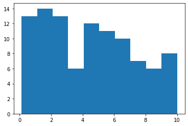
Figure 13: The uniform distribution histogram.
Bernoulli Distribution
Distributions with two outcomes for a random variable are called Bernoulli distributions. It has
one
variable $p$ that indicates the greater probability. $k$ being the possible outcomes, the
probability mass function of the Bernoulli distribution is
\begin{align}
f(k,p) = \left\{
\begin{array}{ll}
p & if\; k=1 \\
q=1-p & if\; k=0
\end{array}
\right.
\end{align}
And it can also be expressed as
\begin{align}
f(k,p)=p^k(1-p)^{1-k}
\end{align}
Expected value of Bernoulli Distribution is $E[X]=p$.
\begin{align}
E[X]&=\sum \:xp\left(x\right)\: \\
&=0.p^0(1-p)^{1-0}+1.p^1(1-p)^{1-1} \\
&=0(1-p)+p \\
&=p
\end{align}
And its variance is $Var(X)=p(1-p)$.
\begin{align}
E[X^2]&=p.1^2+q.0^2 \\
Var(X)&=E[X^2]-E^2[X]=p-p^2=p(1-p)
\end{align}
Bernoulli distribution is denoted by $X\sim Bern(p)$.
Binomial Distribution
To calculate the outcome of more than one Bernoulli trial, the binomial distribution is used.
For
$k$ successful trials in a total of $n$ trials, the probability mass function is given below.
Note
that $B(1,p)=Bern(p)$.
\begin{align}
f(k,n,p)=\binom{n}{k}p^k(1-p)^{n-k}
\end{align}
Since each variable is an equal Bernoulli random variable with $E[X]=p$, the sum of the n trials
simply gives the expected value of the binomial distribution $E[X]=np$. The same is true for the
variance, the variance is $Var(X)=np(1-p)$.
The coin toss is a good example of this distribution. For a coin toss game where heads is
defined as
0 and tails as 1, the histogram for a total of 5 tosses would look like Figure 14.
heads = 1
tails = 0
dataBinomial = np.array([heads, tails, tails, tails, heads])
binomial = pd.DataFrame(dataBinomial)
binomial.plot(kind="hist", legend=False)
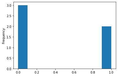
Figure 14: The binomial distribution histogram for a coin toss game.
Python function to calculate binomial distribution for k=7, n=10, and p=0.7 is given below.
from scipy.special import factorial

def nCr(n, r):
return (
factorial(n) / factorial(r) / factorial(n - r)
)  # defining combination formula

def bernouilliPM(k, n, p):
return nCr(n, k) * (p**k * (1 - p) ** (n - k))  # defining bernoulli pm

# the probability of getting 7 successful results in 10 trials with probability of 0.7
bernouilliPM(7, 10, 0.7)
The output is
0.26682793200000005.
Binomial distribution is denoted by $X\sim B(n,p)$.
Poisson Distribution
To find out how often a given event will occur at a given time, the Poison distribution is used.
With $k$ as events, the probability mass function is
\begin{align}
f(k,\lambda)=\frac{\lambda^ke^{-\lambda}}{k!}
\end{align}
The expected value and variance are both equal to $\lambda$: $E[X]=Var(X)=\lambda$.
\begin{align}
E(X)&=\sum_{x=0}^{\infty} x \frac{e^{-\lambda} \lambda^{x}}{x !} \\
&=\sum_{x=1}^{\infty} x \frac{e^{-\lambda} \lambda^{x}}{x !}=\sum_{x=1}^{\infty}
\frac{e^{-\lambda}
\lambda^{x}}{(x-1) !} \\
&=\lambda e^{-\lambda} \sum_{x=1}^{\infty} \frac{\lambda^{x-1}}{(x-1) !} \\
&=\lambda e^{-\lambda} \sum_{x=0}^{\infty} \frac{\lambda^{x}}{x !} \\
&=\lambda e^{-\lambda} e^{\lambda} \\
&=\lambda
\end{align}
For the variance, it is helpful to manipulate the formula $Var(X)=E\left(X^{2}\right)-E(X)^{2}$
by
the following steps.
\begin{align}
&=E((X)(X-1)+X)-E(X)^{2} \\
&=E((X)(X-1))+E(X)-E(X)^{2} \\
&=E((X)(X-1))+\left(\lambda-\lambda^{2}\right)
\end{align}
Replacing,
\begin{align}
&=\sum_{x=0}^{\infty}(x)(x-1) \frac{e^{-\lambda} \lambda^{x}}{x
!}+\left(\lambda-\lambda^{2}\right)
\\
&=\sum_{x=2}^{\infty} \frac{e^{-\lambda} \lambda^{x}}{(x-2) !}+\left(\lambda-\lambda^{2}\right)
\\
&=\lambda^{2} e^{-\lambda} \sum_{x=2}^{\infty} \frac{\lambda^{x-2}}{(x-2)
!}+\left(\lambda-\lambda^{2}\right) \\
&=\lambda^{2} e^{-\lambda} \sum_{x=0}^{\infty} \frac{\lambda^{x}}{x
!}+\left(\lambda-\lambda^{2}\right) \\
&=\lambda^{2} e^{-\lambda} e^{\lambda}+\left(\lambda-\lambda^{2}\right) \\
&=\lambda^{2}+\lambda-\lambda^{2} \\
&=\lambda
\end{align}
The diagram of the probability mass function for various $\lambda$ values can be found in Figure
15.
k = np.arange(0, 10, 1)  # defining the interval
poissonlambda1 = np.exp(-1) * 1**k / factorial(k)
poissonlambda2 = np.exp(-2) * 2**k / factorial(k)
poissonlambda3 = np.exp(-3) * 3**k / factorial(k)
plt.plot(k, poissonlambda1)
plt.plot(k, poissonlambda2)
plt.plot(k, poissonlambda3)
plt.legend(k + 1)  # fixing the legend
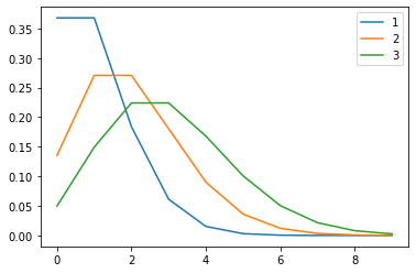
Figure 15: The poisson distribution for $\lambda=\{1,2,3\}$.
Poisson distribution is denoted by $X\sim Po(\lambda)$.
Normal Distribution
Probably the most famous of all distributions, the normal distribution (also known as the
Gaussian
distribution) occupies a very important place in probability theory and statistics because it is
part of the central limit theorem.
The normal distribution is frequently observed in nature. Patterns resulting from biological
events
often form a normal distribution. The probability density function of the normal distribution is
\begin{align}
f\left(x\right)=\frac{1}{\sigma \sqrt{2\pi }}e^{-\frac{1}{2}\left(\frac{x-\mu \:}{\sigma
\:}\right)^2}
\end{align}
For fixed $\mu=0$ and $\sigma^2=\{0.5,1,2\}$ values, the probability density function behaves
like
in Figure 16.
x = np.arange(-5, 5, 0.01)  # setting a range
normalsigmasq05 = (1 / (0.5 * np.sqrt(2 * np.pi))) * np.e ** (
(-1 / 2) * ((x - 0) / 0.5) ** 2
)
normalsigmasq1 = (1 / (1 * np.sqrt(2 * np.pi))) * np.e ** (
(-1 / 2) * ((x - 0) / 1) ** 2
)
normalsigmasq2 = (1 / (2 * np.sqrt(2 * np.pi))) * np.e ** (
(-1 / 2) * ((x - 0) / 2) ** 2
)  # replacing mu with 0 and variance with 0.5,1,2
plt.plot(x, normalsigmasq05)
plt.plot(x, normalsigmasq1)
plt.plot(x, normalsigmasq2)
legend = ("var=0.5", "var=1", "var=2")
plt.legend(labels=legend)
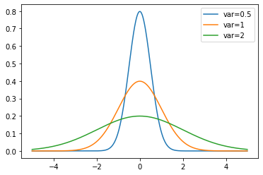
Figure 16: The normal distribution for $mu=0$ and $\sigma^2=\{0.5,1,2\}$.
The normal distribution is clearly a continuous distribution and the expected value for continuous
distributions is calculated with the following formula:
\begin{align}
\mathrm{E}[\mathrm{X}]=\int_{-\infty}^{\infty} x f(x) d x
\end{align}
Replacing
\begin{align}
E\left(X\right)&=\int _{-\infty }^{\infty }x\frac{1}{\sigma\sqrt{2\pi
}}e^{-\frac{1}{2}\left(\frac{x-\mu
}{\sigma}\right)^2}dx \\
&=\frac{1}{\sigma\sqrt{2\pi }}\int _{-\infty }^{\infty }xe^{-\frac{1}{2}\left(\frac{x-\mu
}{\sigma}\right)^2}dx
\end{align}
Changing the variable as $t=\frac{x-\mu}{\sqrt{2}\sigma}$, gives $x=\mu+\sqrt{2}\sigma t$ and
$dx=\sqrt{2}\sigma dt$. Replacing again,
\begin{align}
E\left(X\right)&=\frac{1}{\sigma\sqrt{2\pi}}\int _{-\infty }^{\infty }\left(\mu +\sqrt{2}\sigma t
\right)e^{-t^2}\sqrt{2}\sigma dt \\
&=\frac{1}{\sqrt{\pi }}\int _{-\infty }^{\infty }\left(\mu +\sqrt{2}\sigma t \right)e^{-t^2}dt
\end{align}
Splitting the integral into sums and solving them
\begin{align}
&=\frac{1}{\sqrt{\pi}}\left[\mu\int _{-\infty }^{\infty }e^{-t^2}dt+\sqrt{2}\sigma\int
_{-\infty}^{\infty}te^{-t^2}dt\right] \\
&=\frac{1}{\sqrt{\pi}}\left[\mu\sqrt{\pi }+\sqrt{2}\sigma \left(-\frac{1}{2}e^{-t^2}\right)_{-\infty
}^{\infty }\right] \\
&=\frac{1}{\sqrt{\pi}}\left[\mu \sqrt{\pi}+0\right] \\
&=\mu
\end{align}
The expected value of the normal distribution is $\mu$.
To find the variance of the normal distribution, we start with $Var(X)=E[X^2]-E^2[X]`. Since
$E[X]=\mu$,
the formula becomes $Var(X)=E[X^2]-\mu^2$.
\begin{align}
E[X^2]&=\int _{-\infty }^{\infty }x^2\frac{1}{\sigma\sqrt{2\pi }}e^{\frac{-\left(x-\mu
\right)^2}{2\sigma ^2}}dx-\mu ^2 \\
&=\frac{1}{\sigma \sqrt{2 \pi}} \int_{-\infty}^{\infty} x^{2} e^{\frac{-(x-\mu)^{2}}{2 \sigma^{2}}}
d
x-\mu^{2}
\end{align}
With the same substitution $t=\frac{x-\mu}{\sqrt{2}\sigma}$
\begin{align}
&=\frac{1}{\sigma \sqrt{2 \pi}} \int_{-\infty}^{\infty}(\sqrt{2} \sigma t+\mu)^{2} e^{-t^{2}}
\sqrt{2}
\sigma d t-\mu^{2} \\
&=\frac{1}{\sqrt{\pi}} \int_{-\infty}^{\infty}(\sqrt{2} \sigma t+\mu)^{2} e^{-t^{2}} d t-\mu^{2} \\
&=\frac{1}{\sqrt{\pi}}\left[\int_{-\infty}^{\infty}\left(2 \sigma^{2} t^{2}+2 \sqrt{2} \sigma \mu
t+\mu^{2}\right) e^{-t^{2}} d t\right]-\mu^{2} \\
&=\frac{1}{\sqrt{\pi}}\left[2 \sigma^{2} \int_{-\infty}^{\infty} t^{2} e^{-t^{2}} d t+2 \sqrt{2}
\sigma
\mu \int_{-\infty}^{\infty} t e^{-t^{2}} d t+\mu^{2} \int_{-\infty}^{\infty} e^{-t^{2}} d
t\right]-\mu^{2} \\
&=\frac{1}{\sqrt{\pi}}\left[2 \sigma^{2} \int_{-\infty}^{\infty} t^{2} e^{-t^{2}} d t+2 \sqrt{2}
\sigma
\mu .0+\mu^{2} \sqrt{\pi}\right]-\mu^{2} \\
&=\frac{1}{\sqrt{\pi}}\left[2 \sigma^{2} \int_{-\infty}^{\infty} t^{2} e^{-t^{2}} d
t\right]+\frac{1}{\sqrt{\pi}} \mu^{2} \sqrt{\pi}-\mu^{2} \\
&=\frac{2 \sigma^{2}}{\sqrt{\pi}} \int_{-\infty}^{\infty} t^{2} e^{-t^{2}} d t \\
\end{align}
Integrating by parts
\begin{align}
&=\frac{2 \sigma^{2}}{\sqrt{\pi}}\left(\left[-\frac{t}{2}
e^{-t^{2}}\right]_{-\infty}^{\infty}+\frac{1}{2} \int_{-\infty}^{\infty} e^{-t^{2}} d t\right) \\
&=\frac{2 \sigma^{2}}{\sqrt{\pi}}\left(0+\frac{1}{2} \int_{-\infty}^{\infty} e^{-t^{2}} d t\right)
\\
&=\frac{\sigma^{2}}{\sqrt{\pi}} \int_{-\infty}^{\infty} e^{-t^{2}} d t \\
&=\frac{\sigma^{2}}{\sqrt{\pi}} \sqrt{\pi} \\
&=\sigma^{2}
\end{align}
As calculated above, variance of the normal distribution is $\sigma^2$.
Normal distribution is denoted by $X\sim N(\mu,\sigma^2)$.
Standard Normal Distribution
The normal distribution with mean $\mu=0$ and variance $\sigma^2=1$ is called the standard
normal
distribution.
The normal distribution can be standardized with the following formula
\begin{align}
z=\frac{x-\mu}{\sigma}
\end{align}
With this transformation, we obtain the variable $z$, that is, the standard deviations between
the
values and the mean. Then the z-table is used to find the percentage of variables that are
distributed above or below $x$.
The plot of the probability density function of the standard normal distribution can also be
seen in
Figure 16.
Standard normal distribution is denoted by $Z\sim N(0,1)$.
normalization and Standardization
For some models to work properly, the data must be normalized or standardized. Both are methods
of
scaling features that differ from each other in some respects.
Normalization is often used when the distribution of the data is unknown. To determine the
normalized value, the minimum and maximum values are needed.
\begin{align}
X_{\text {normalized }}=\frac{X-X_{\min }}{X_{\max }-X_{\min }}
\end{align}
Normalized values have a predefined range that lies between $[-1, 1]$ or $[0, 1]$, which means
that
it is affected by outliers. With standardization, on the other hand, this is not the case, since
the
standard distribution has no defined range.
Standardization is useful when the data are normally distributed. After the following
transformation, the mean is set to 0 and the variance is set to 1.
\begin{align}
z=\frac{x-\mu}{\sigma}
\end{align}
Student's T Distribution
Published by William Sealy Gosset under the
pseudonym "Student" (because the company he works for did not allow its scientists to
use their real names in publications (Raju, 2005)),Student's T distribution can be defined as an
approximation to the normal distribution for limited data. This distribution has its own
cumulative
table, like the z-table used in the standard normal distribution, and it is called the t-table.
Student's T distribution is used for small samples with unknown variances, while the standard
normal
distribution is used for large samples with known variances. $\nu$ in $X\sim t(\nu)$ represents
degrees of freedom, calculated with $\nu=n-1$, where $n$ is the number of observations in the
sample. If $\nu > 2$, expected value $E[X]=\mu$ and $Var(X)=\frac{S^2k}{k-2}$, where $S^2$ is
the
variance of the sample.
$\Gamma$ is the gamma function, the probability density function of Student's T distribution is
\begin{align}
f(x, \nu)=\frac{\Gamma((\nu+1) / 2)}{\sqrt{\pi \nu} \Gamma(\nu / 2)}\left(1+x^{2} /
\nu\right)^{-(\nu+1) / 2}
\end{align}
Below is a Python code to compare Student's T with the standard normal distribution with $\nu=1$
and
$\nu=2$. See Figure 17.
x = np.arange(-5, 5, 0.01)  # setting a range
plt.plot(x, stats.norm.pdf(x, 0, 1))
plt.plot(x, stats.t.pdf(x, 1))
plt.plot(x, stats.t.pdf(x, 2))
legend = ("std normal", "stu t, nu=1", "stu t, nu=2")
plt.legend(labels=legend)
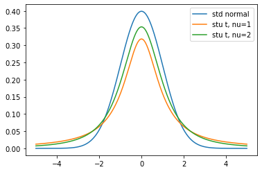
Figure 17: Student's T with $\nu=1, \: 2$ and standard normal. Notice the higher tails on
Student's T.
One can see that with higher degrees in freedom, Student's T converges to standard normal.
Student's T distribution is denoted by $X\sim t(\nu)$.
Chi-Squared Distribution
The chi-square distribution is one of the most commonly used probability distributions, which
has
little application in real life but plays an important role in hypothesis testing. It is
obtained by
summing the squares of $k$ standard normally distributed random variables, where $k$ is the
degrees
of freedom. The expected value of the chi-squared distribution is $E[X]=k$ and the variance is
$Var(X)=2k$. The probability density function of this distribution is
\begin{align}
f(x, k)=\frac{1}{2^{k / 2} \Gamma(k / 2)} x^{k / 2-1} e^{(-x / 2)}
\end{align}
Here is a graph to compare between different $k$ values. As with Student's T, the diagram
converges
to the normal distribution at higher degrees of freedom. See Figure 18.
x = np.arange(0, 10, 0.01)  # setting a range
k = np.arange(1, 8, 1)
legend = []

for df in k:  # plotting k values from 1 to 7
plt.plot(x, stats.chi2.pdf(x, df))
legend.append(f"k={df}")

plt.axis([0, 10, 0, 0.5])  # setting graph limits
plt.legend(labels=legend)
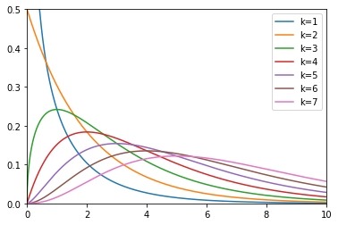
Figure 18: The chi-squared distribution with different degrees of freedom.
The chi-squared distribution is denoted by $X\sim \chi^2(k)$.
Exponential Distribution
Like the chi-squared distribution, the exponential distribution is a special case of the gamma
distribution. Variables that follow the exponential distribution start with high probability,
decrease, and eventually reach a plateau. $\lambda$ in $X\sim exp(\lambda)$ is defined as rate
parameter. It indicates how fast the probability density function reaches the plateau and how
spread
the graph is. The probability density function is
\begin{align}
f(x ; \lambda)=\left\{\begin{array}{ll}
\lambda e^{-\lambda x} & x \geq 0 \\
0 & x \lt 0
\end{array}\right.
\end{align}
For the distribution graph, see Figure 19.
x = np.arange(0, 10, 0.01)
rate = np.arange(0.5, 2.5, 0.5)
legend = []

for lamb in rate:
plt.plot(x, lamb * np.exp(-lamb * x))
legend.append(f"lambda={lamb}")

plt.axis([0, 5, 0, 1.5])
plt.legend(labels=legend)
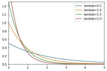
Figure 19: The exponential distribution with different rate parameters.
The exponential distribution is denoted by $X\sim exp(\lambda)$.
Logistic Distribution
The logistic distribution is often used to determine how continuous variables affect the
probability
of Boolean outcomes. $\mu$ in $X\sim logistic(\mu,S)$ represents location and $S$ represents
scale.
The scale determines how wide the bell curve is.
The probability density function of the logistic distribution
\begin{align}
f(x ; \mu, s)=\frac{e^{-(x-\mu) / s}}{s\left(1+e^{-(x-\mu) / s}\right)^{2}}
\end{align}
is also equal to
\begin{align}
=\frac{1}{4 s} \operatorname{sech}^{2}\left(\frac{x-\mu}{2 s}\right)
\end{align}
The probability density function looks like a normal distribution but has a lower tail. See
Figure
20.
x = np.arange(-10, 20, 0.01)
mu = [2, 9]
s = [2, 3]
legend = []

for location in mu:
for scale in s:
plt.plot(
    x,
    (np.exp(-(x - location) / scale))
    / (scale * (1 + np.exp(-(x - location) / scale)) ** 2),
)
legend.append(f"mu={location},s={scale}")

plt.legend(labels=legend)
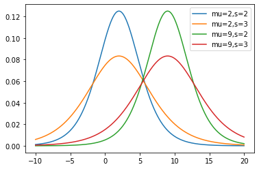
Figure 20: The logistic distribution with different location and scale parameters.
The expected value of the logistic distribution is $E[X]=\mu$ and the variance is
$Var(X)=\frac{s^2\pi^2}{3}$.
The logistic distribution is denoted by $X\sim logistic(\mu, S)$.
Statistics
Statistics is based on probability theory and is used for sampling and inference in the most
general sense. Various statistical measures help to identify the structure of the sample,
while inferential statistics aim to infer properties from the data when descriptive statistics
are not sufficient. This section includes these two topics as main headings.
Statistics is the cornerstone of data science, it is impossible to distinguish them. Even
more, statistics occupies such an important place in data science that scholars once argued
about whether or not statistics should be called data science (Diggle, 2015).
Measures
In statistics, different types of measurement methods are used to determine the behaviour of
data.
These methods are used to find out how the sample behaves around the centre, how skewed it is,
how
much variability it has, or how different variables affect each other. Four types of statistical
measurement methods play an important role, especially in machine learning.
Measures of Central Tendency
The measure of central tendency, one of the most fundamental concepts in statistics, gives the
average of the sample in different approaches.
Mean
The mean is the average of the data. The population mean is denoted with $\mu$ and calculated with
\begin{align}
\mu=\frac{\sum_{i=1}^nx_i}{n}
\end{align}
while the sample mean is denoted by $\bar{x}$, and calculated with
\begin{align}
\bar{x}=\frac{\sum_{i=1}^Nx_i}{N}
\end{align}
The mean is easily affected by the outliers.
Median
The median is the number in the middle of the sorted data.
Mode
The mod is the number that most occurs in the data set.
Mean, median, and mode needed to be used together to get enough conclusions about the data.
Measures of Asymmetry
Asymmetry measures are used to examine whether a data set has an unequal distribution on
opposite
sides of the mean.
Skewness
Indicates if the data is distributed unevenly on a side or not. Skewness is calculated with
\begin{align}
\frac{\frac{1}{n} \sum_{i=1}^{n}\left(x_{i}-\bar{x}\right)^{3}}{\sqrt{\frac{1}{n-1}
\sum_{i=1}^{n}\left(x_{i}-\bar{x}\right)^{2}}^{3}}
\end{align}
Three different types skewness can be observed
- When the mean is greater than the median, the distribution has positive (right) skewness.
- If the mean is equal to the median, the distribution has no skewness, i.e., it is symmetric.
- If the mean is smaller than the median, the distribution has negative (left) skew.
Measures of Variability
Measures of variability illustrate the irregularities in a data set. The lower the values of the
variability measure, the more similar the data values are in a set.
Variance
Variance indicates how much the data deviates from the mean. The variance of the population is
denoted by $\sigma^2$. It is one of the basic measures along with the expected value. The
population
variance is calculated with
\begin{align}
\sigma^{2}=\frac{\sum_{i=1}^{N}\left(x_{i}-\mu\right)^{2}}{N}
\end{align}
And the sample variance is denoted with $s^2$, it is calculated with
\begin{align}
s^{2}=\frac{\sum_{i=1}^{n}\left(x_{i}-\bar{x}\right)^{2}}{n-1}
\end{align}
Standard Deviation
The standard deviation is the square root of the variance and is used for the same purpose. The
variance is squared to amplify the effect of large differences. The standard deviation of a
population is denoted by $\sigma$, and is calculated as follows.
\begin{align}
\quad \sigma=\sqrt{\frac{\sum_{i=1}^{N}\left(x_{i}-\mu\right)^{2}}{N}}
\end{align}
Meanwhile the sample standard deviation is denoted with $s$, and is calculated with
\begin{align}
\quad S=\sqrt{\frac{\sum_{i=1}^{n}\left(x_{i}-\bar{x}\right)^{2}}{n-1}}
\end{align}
Coefficient of Variation
The coefficient of variation is used for comparison purposes. It is determined by dividing the
standard deviation by the mean and has no unit of measurement. The coefficient of variation of
the
population is
\begin{align}
C_v=\frac{\sigma}{\mu}
\end{align}
And the coefficient of variation of the sample is
\begin{align}
\hat{C_v}=\frac{s}{\bar{x}}
\end{align}
Measures of Relationship Between Variables
Relationship measures are used to discover the relationships between different variables. Higher
values of the relationship measure are more likely to move the variables together.
Covariance
Covariance is the measure of mutual variability. The covariance of a population is calculated
according to the following formula
\begin{align}
\sigma_{x y}=\frac{\sum_{i=1}^{N}\left(x_{i}-\mu_{x}\right) *\left(y_{i}-\mu_{y}\right)}{N}
\end{align}
And the sample covariance is calculated with
\begin{align}
\quad S_{x y}=\frac{\sum_{i=1}^{n}\left(x_{i}-\bar{x}\right) *\left(y_{i}-\bar{y}\right)}{n-1}
\end{align}
- A positive covariance means that the variables grow in the same direction.
- A negative covariance means that the variables grow in the opposite direction.
- A covariance of zero means that the variables are independent.
Note that $Cov(x,y)=E[xy]-E[x]E[y]$. Thus, if $x=y$, $Cov(x,x)=E[xx]-E[x]E[x]$ means that
$Cov(x,x)=Var(x)$.
Correlation
Correlation is the normalized version of covariance. Covariance can take any value, while
correlation can take values between -1 and 1. The population correlation is calculated with
\begin{align}
\rho=\frac{\sigma_{x y}}{\sigma_{x} \sigma_{y}}
\end{align}
And the sample correlation is calculated with
\begin{align}
\mathrm{r}=\frac{s_{x y}}{s_{x} s_{y}}
\end{align}
- If the correlation is equal to 1, there is a perfect correlation. One variable can be fully
explained by the other variable.
- If the correlation is equal to 0, there is no commonality between the variables.
- If the correlation is equal to -1, there is a perfect negative correlation. This means that
the
relationship between the variables is always opposite.
It is crucial to know that correlation does not imply causation.
Inferential Statistics
Statistics is about collecting data and drawing inferences from the sample. Inferential
statistics
is a branch of statistics that focuses on this purpose. Methods such as parameter estimation and
hypothesis testing can be used to generalize data to make predictions using the central limit
theorem, which is proved using the weak law of large numbers.
Central Limit Theorem
The weak law of large numbers states that for a sufficiently large sample, the sample mean
$M_{n}$
converges to the true mean $\mu$ and can also be expressed as follows: It is unlikely that the
sample mean $M_{n}$ deviates far from the true mean $\mu$.
Let $x_1,x_2,...$ be independent and identically distributed random variables with finite mean
$\mu$
and variance $\sigma^2$. Then the sample mean is
\begin{align}
M_n=\frac{x_1+...+x_n}{n}
\end{align}
To implement Markov's inequality, the expected value and the variance of $M_n$ must first be
calculated.
\begin{align}
E[M_n]&=\frac{E[x_1+...+x_n]}{n}=\frac{n\mu}{n}=\mu \\
Var(M_n)&=\frac{Var(x_1+...+x_n)}{n^2}=\frac{n\sigma^2}{n^2}=\frac{\sigma^2}{n}
\end{align}
For a fixed $\epsilon>0$,
\begin{align}
P(|M_n-\mu|\geq\epsilon)\leq\frac{Var(M_n)}{n\epsilon^2}\xrightarrow[n\rightarrow\infty]{}0
\end{align}
In conclusion,
\begin{align}
\text{For} \:\:\epsilon>0,
\:P(|M_n-\mu|\geq\epsilon)=P(|\frac{x_1+...+x_n}{n}-\mu|\geq\epsilon)\rightarrow0\:\:\text{as}\:\:n\rightarrow\infty
\end{align}
The central limit theorem states that for any distribution, the sample distribution of the mean
converges to the normal distribution.
Let $x_1,x_2,...$ be independent and identically distributed random variables with finite mean
$\mu$
and variance $\sigma^2$.
\begin{align}
Z=\frac{x_1+x_2+...+x_n-n\mu}{\sigma\sqrt{n}}
\end{align}
tends to standard normal as $n\rightarrow\infty$.
\begin{align}
P\{ \frac{x_1+x_2+...+x_n-n\mu}{\sigma\sqrt{n}}\leq a \}\rightarrow \int _{-\infty
}^0e^{-x^2/2}dx\:\:\text{as}\:\:n\rightarrow\infty
\end{align}
Standard Error
The standard error is the standard deviation of the sampling distribution. It indicates the
variability of a sample, as does any standard deviation. It is calculated with the formula
\begin{align}
\sqrt{\frac{\sigma^2}{n}}=\frac{\sigma}{\sqrt{n}}
\end{align}
where
\begin{align}
\text{Sampling distribution} \sim N\left(\mu,\frac{\sigma^2}{n}\right)
\end{align}
The standard error decreases with decreasing sample size, since it is easier to find the true
mean
with smaller samples.
Estimators
Population parameters such as mean ($\mu$), variance ($\sigma^2$), and correlation ($\rho$) are
approximated from the sample using functions called estimators. The mean estimator is denoted by
$\bar{x}$, while the variance estimator is denoted by $s^2$ and the correlation estimator by
$r$.
An unbiased estimator with minimum variance is considered an optimal estimator. The bias of an
estimator is the difference between the parameter and the estimate. Consider a variance estimate
that results as $\sigma^2 + b$, $b$ here is the bias. Note that an unbiased estimator perfectly
approximates the population parameter.
Estimates
Values obtained from estimators are called estimates. Point estimates output a single value,
while
confidence intervals output an interval. It is safer to use confidence intervals than point
estimates.
The confidence level is calculated as $(1-\alpha)$. Conventional values for $\alpha$ are $0.01$,
$0.05$, and $0.1$. Confidence intervals indicate that the estimated parameter is certain to be
within the calculated range and are calculated using the following formulas.
For a single population, if the variance is known, the $z$ statistic is used. Hence the variance
is
equal to $\sigma^2$. The confidence interval is calculated using
\begin{align}
\bar{x} \pm z_{\alpha / 2} \frac{\sigma}{\sqrt{n}}
\end{align}
And if the variance is unknown, the $t$ statistic is used. Thus the variance is $s^2$. The
confidence interval is
\begin{align}
\bar{x} \pm t_{n-1, \alpha / 2} \frac{s}{\sqrt{n}}
\end{align}
For two populations with dependent samples, the $t$ statistic is used as well. Here, the
variance is
$s_{\text {difference }}^{2}$ and the confidence interval is
\begin{align}
\overline{\mathrm{d}} \pm t_{n-1, \alpha / 2} \frac{s_{d}}{\sqrt{n}}
\end{align}
The $z$ statistic is used for two populations with known variances and independent samples. The
variances are $\sigma_{x}^{2}$ and $\sigma_{y}^{2}$, while the confidence interval is
\begin{align}
(\bar{x}-\bar{y}) \pm z_{\alpha / 2}
\sqrt{\frac{\sigma_{x}^{2}}{n_{x}}+\frac{\sigma_{y}^{2}}{n_{y}}}
\end{align}
When the variance is unknown but considered equal for two populations with independent samples,
the
$t$ statistic is used. Therefore, the variance is equal to
\begin{align}
s_{p}^{2}=\frac{\left(n_{x}-1\right) s_{x}^{2}+\left(n_{y}-1\right) s_{y}^{2}}{n_{x}+n_{y}-2}
\end{align}
and the confidence interval is calculated using the formula
\begin{align}
(\bar{x}-\bar{y}) \pm t_{n_{x}+n_{y}-2, \alpha / 2}
\sqrt{\frac{s_{p}^{2}}{n_{x}}+\frac{s_{p}^{2}}{n_{y}}}
\end{align}
When the variance is unknown but considered different for two populations with independent
samples,
the $t$ statistic is also used. The variances are equal to $s_{x}^{2}$ and $s_{y}^{2}$, and the
confidence interval is
\begin{align}
(\bar{x}-\bar{y}) \pm t_{\mathrm{v}, \alpha / 2}
\sqrt{\frac{s_{x}^{2}}{n_{x}}+\frac{s_{y}^{2}}{n_{y}}}
\end{align}
Hypothesis Testing
Hypothesis testing is a statistical method used to determine whether the hypothesis made about
the
sample is true. The hypothesis to be
tested is called the null hypothesis, and the possible conditions of the null hypothesis can
be seen in Table 3. Note the similarities between the confusion matrix.
|
Truth |
|
| Decision |
$H_0$ is true |
$H_0$ is false |
| Accept $H_0$ |
Confidence level $(1 - \alpha )$ |
Type II error $(\beta)$ |
| Reject $H_0$ |
Type I error $(\alpha)$ |
Power $(1 - \beta )$ |
Table 3: The hypothesis testing table.
Another name for the type I error is significance level (Gustafsen, 2022). The minimum
value for the significance level to reject the null hypothesis is called the p-value. The
desired values for the p-value are close to 0. The null hypothesis is rejected if the test
statistic
is greater than the critical value. The formulas for the test statistic for different
conditions are given below.
For a population with known variance, the formula for the test statistic is
\begin{align}
Z=\frac{\bar{x}-\mu_{0}}{\sigma / \sqrt{\mathrm{n}}}
\end{align}
And with unknown variance, the formula becomes
\begin{align}
T=\frac{\bar{x}-\mu_{0}}{s / \sqrt{n}}
\end{align}
For two populations with dependent samples, the test statistic is
\begin{align}
T=\frac{\bar{d}-\mu_{0}}{s_{d} / \sqrt{n}}
\end{align}
For two populations with independent samples, the formula for the test statistic when the
variance
is
known is
\begin{align}
Z=\frac{(\bar{x}-\bar{y})-\mu_{0}}{\sqrt{\frac{\sigma_{x}^{2}}{n_{x}}+\frac{\sigma_{y}^{2}}{n_{y}}}}
\end{align}
And for two populations with independent samples, when the variance is unknown but considered
equal,
the
test statistic is
\begin{align}
T=\frac{(\bar{x}-\bar{y})-\mu_{0}}{\sqrt{\frac{s_{p}^{2}}{n_{x}}+\frac{s_{p}^{2}}{n_{y}}}}
\end{align}
Conclusion
Artificial intelligence is a subfield of data science and closely related to statistics.
Artificial
intelligence algorithms learn, in a sense, by optimizing themselves with respect to the goal to
be
achieved, and the trained models are used to make predictions. It is not surprising that
artificial
intelligence is now appearing in every field where predictions are made. This field, which is
growing in popularity, continues to fascinate us with its findings.
The information obtained in this study not only provides a foundation for machine learning, but
may
also lead to the discovery of new methods. It is difficult to predict what the future will
bring,
but given the rapid pace of recent developments, it is obvious that we will see many more
exciting
innovations. The most important thing is that we use them for the benefit of humanity.
References
-
AlphaZero: Shedding new light on the grand games of chess, shogi and Go. (n.d.). Retrieved
2022-01-09, from
https://deepmind.com/blog/article/alphazero-shedding-new-light-grand-games-chess-shogi-and-go
-
Arsht, E. (2019, April). Napoleon was the best general ever, and the math proves it.
Retrieved
2022-01-05, from
https://towardsdatascience.com/napoleon-was-the-best-general-ever-and-the-math-proves-it-86efed303eeb
-
Bayes’ theorem. (2022). Retrieved 2022-06-12, from
https://corporatefinanceinstitute.com/resources/knowledge/other/bayes-theorem/
-
Bloomfield, P. (2004). Fourier analysis of time series: an introduction. John Wiley & Sons.
-
Brownlee, J., Cristina, S., & Saeed, M. (2022). Calculus for machine learning. Machine
Learning
Mastery.
-
Cao, L. (2017). Data science: a comprehensive overview. ACM Computing Surveys (CSUR), 50(3),
1-42.
-
DasGupta, A. (2011). Probability for statistics and machine learning: fundamentals and
advanced
topics. Springer.
-
Diggle, P. J. (2015). Statistics: a data science for the 21st century. Journal of the Royal
Statistical Society: Series A (Statistics in Society), 178(4), 793–813.
-
Garding, L., & Tambour, T. (2012). Algebra for computer science. Springer Science & Business
Media.
-
Glorot, X., & Bengio, Y. (2010). Understanding the difficulty of training deep feedforward
neural networks. In Proceedings of the thirteenth international conference on artificial
intelligence and statistics (pp. 249-256).
-
Gustafsen, A. (2022, March). The confusion matrix in hypothesis testing. Retrieved
2022-06-15,
from
https://towardsdatascience.com/the-confusion-matrix-explained-part-1-5513c6f659c1
-
Holbrook, R. (2021). Time series tutorials. Retrieved 2022-06-03, from
https://www.kaggle.com/learn/time-series
-
Kan, E. (2021, August). Quick ml concepts: tensors. Retrieved 2022-06-16, from
https://towardsdatascience.com/quick-ml-concepts-tensors-eb1330d7760f
-
Kumar, P. (2021, June). Time complexity of ml models. Retrieved 2022-06-17, from
https://medium.com/analytics-vidhya/time-complexity-of-ml-models-4ec39fad2770
-
Lydia, A., & Francis, S. (2019). Adagrad—an optimizer for stochastic gradient descent. Int.
J.
Inf. Comput. Sci, 6(5), 566-568
-
Okewu, E., Misra, S., & Lius, F.-S. (2020). Parameter tuning using adaptive moment
estimation in
deep learning neural networks. In International conference on computational science and its
applications (pp. 261-272).
-
Rajendran, P. K., Asbern, A., Kumar, K. M., Rajesh, M., & Abhilash, R. (2016).
Implementation
and analysis of mapreduce on biomedical big data. Indian Journal of Science and Technology,
9(31).
-
Raju, T. N. (2005). William sealy gosset and william a. silverman: two “students” of
science.
Pediatrics, 116(3), 732-735.
-
Rosenthal, A. (1951). The history of calculus. The American Mathematical Monthly, 58(2),
75-86.
-
Shafi. (2020, October). Ai & mathematics. Retrieved 2022-06-18, from
https://medium.com/swlh/ai-mathematics-699a9ea2a0d6
-
Steinke, S. (2017, August). What’s the difference between a matrix and a tensor? Retrieved
2022-06-17, from
https://medium.com/@quantumsteinke/whats-the-difference-between-a-matrix-and-a-tensor-4505fbdc576c
-
The Editors of Encyclopaedia Britannica. (2020). Digital computer | evolution, components, &
features | britannica. Retrieved 2022-06-17, from
https://www.britannica.com/technology/digital-computer
-
vartika02. (2019, January). 5 V’s of Big Data. Retrieved 2021-12-29, from
https://www.geeksforgeeks.org/5-vs-of-big-data/
-
Xu, D., & Tian, Y. (2015). A comprehensive survey of clustering algorithms. Annals of Data
Science, 2(2), 165-193.